The Fin Problem
I recently wrote about my research on fins and I think I should take some time to write more about the mathematical aspect of it.
In this post, I will write about the solution to a 2D fin. In the previous post, I gave the solution to the 1D fin, so I won’t be going over it again.
The Problem Statement
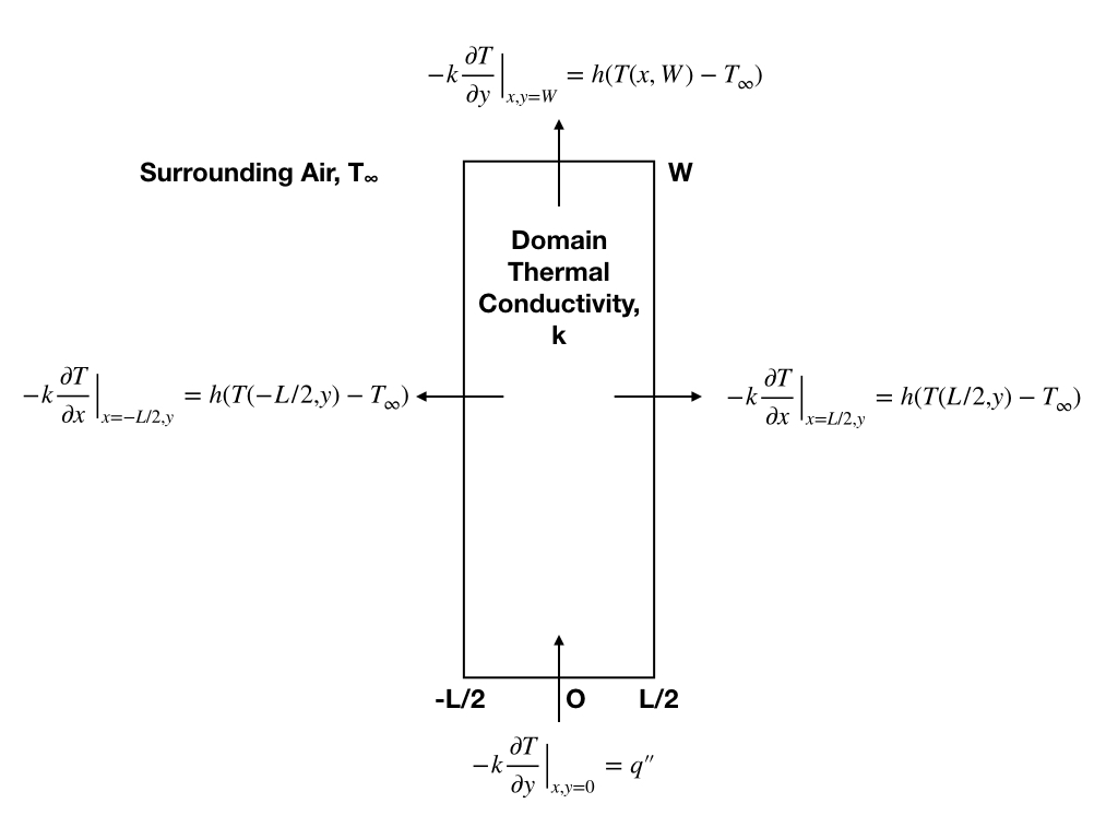
The problem is described in the previous post. I will describe it here once again. A rectangular fin has the dimensions LxW. It is heated from the bottom with a constant heat flux of \( q’'\). The other surfaces are losing heat to surrounding through via convection. The heat transfer coefficient \( h\) is assumed to be a constant. Surrounding air is at temperature \( T_{\infty}\).
 |
Solution:
To solve this problem, first let us look at the boundary conditions on each of the domain boundaries. The bottom boundary is a non-homogenous boundary with constant heat flux. The left and right boundaries are identical, and are non-homogenous convective boundaries. The top boundary is a non-homogenous convective boundary.
From the Strum-Liouville post, we know that we can solve for one non-homogenous boundary. Now since we have 4 non-homogenous boundaries, the solution to the problem will be extremely difficult.
But once again, math provides us with some elegant solutions. In the above problem, the governing equation within the domain is given by:
\[ \dfrac{\partial^2 T}{\partial x^2} + \dfrac{\partial^2 T}{\partial y^2} = 0\]
OR
\[ \nabla^2 T = 0\]
The Laplace equation is a second order linear differential equation. Due to its linear nature, we can superimpose solutions to sub-problems to obtain a global solution.
Before we break down our problem, let us make a small simplification. Since the problem is symmetric in the X-direction, we will only solve for the positive half. The negative half will be a mirror image of this solution. Thus, the updated boundary condition will be \( \dfrac{\partial T}{\partial x} \bigr\vert_{x=0,y}= 0\).
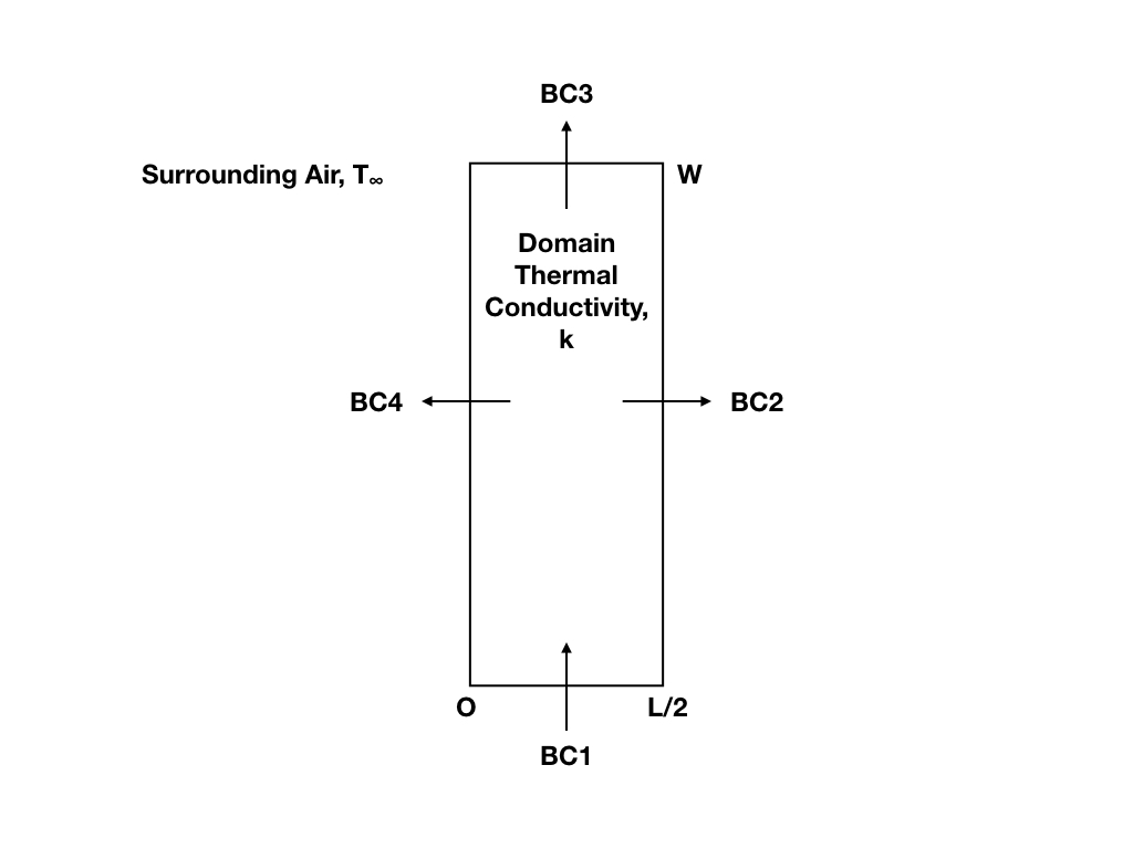 |
In the above diagram, for the full problem the boundary conditions are given by:
BC1: \( -k\dfrac{\partial T}{\partial y} \bigr\vert_{x,y=0} = q’'\)
BC2: \( -k\dfrac{\partial T}{\partial x} \bigr\vert_{x=L/2,y} = h(T(L/2,y) - T_{\infty})\)
BC3: \( -k\dfrac{\partial T}{\partial y} \bigr\vert_{x,y=W} = h(T(x,W)-T_{\infty})\)
BC4: \( \dfrac{\partial T}{\partial x} \bigr\vert_{x=0,y} = 0\)
Now, let us break the problem down into 4 parts such that each time, one of the boundary condition is the non-homogenous one, and all other boundaries are homogeneous while maintaining the type of boundary. Thus, if one of the boundaries was a Dirichlet boundary, we would ensure that the homogeneous one would also be a Dirichlet boundary. Similarly for Neumann boundaries. In the case of mixed boundaries, we ensure that the non-homogeneous part is put to 0. E.g., in the above case, we would make \( T_{\infty} = 0\) to convert the boundary to a homogenous boundary.
Part 1: BC1 is non-homogeneous
We have,
\[ \dfrac{\partial^2 T_1}{\partial x^2} + \dfrac{\partial^2 T_1}{\partial y^2} = 0\]
Subject to:
BC1: \( -k\dfrac{\partial T_1}{\partial y} \bigr\vert_{x,y=0} = q’'\)
BC2: \( -k\dfrac{\partial T_1}{\partial x} \bigr\vert_{x=L/2,y} = h(T_1(L/2,y))\)
BC3: \( -k\dfrac{\partial T_1}{\partial y} \bigr\vert_{x,y=W} = h(T_1(x,W))\)
BC4: \( \dfrac{\partial T_1}{\partial x} \bigr\vert_{x=0,y} = 0\)
Let \( T_1(x,y) = X_1(x).Y_1(y)\) as before. Thus,
\[ \dfrac{1}{Y_1} . \dfrac{\partial^2 Y_1}{\partial y^2} = -\dfrac{1}{X_1} . \dfrac{\partial^2 X_1}{\partial x^2} = \lambda^2\]
\[ \therefore \dfrac{\partial^2 Y_1}{\partial y^2} - \lambda^2 Y_1 = 0\] and
\[ \dfrac{\partial^2 X_1}{\partial x^2} + \lambda^2 X_1 = 0\]
\[ \therefore X_1 = C_1\cos(\lambda x) + C_2\sin(\lambda x)\]
\[ \therefore Y_1 = C_3\cosh(\lambda y) + C_4\sinh(\lambda y)\]
\[ \therefore T_1(x,y) = (C_1\cos(\lambda x) + C_2\sin(\lambda x))(C_3\cosh(\lambda y) + C_4\sinh(\lambda y))\]
Now, let us satisfy the boundary conditions one by one. We will deal with the non-homogenous boundary at the end.
\[ \dfrac{\partial T_1}{\partial x} = (-C_1\lambda\sin(\lambda x) + C_2\lambda\cos(\lambda x))(C_3\cosh(\lambda y) + C_4\sinh(\lambda y))\]
\[ \dfrac{\partial T_1}{\partial y} = (C_1\cos(\lambda x) + C_2\sin(\lambda x))(C_3\lambda\sinh(\lambda y) + C_4\lambda\cosh(\lambda y))\]
Starting with BC4,
\[ \dfrac{\partial T_1}{\partial x} \bigr\vert_{x=0,y} = 0\]
\[ (C_2\lambda)(C_3\cosh(\lambda y) + C_4\sinh(\lambda y)) = 0 \Rightarrow C_2 = 0\]
Now, resolving BC2,
\[ -k\dfrac{\partial T_1}{\partial x} \bigr\vert_{x=L/2,y} = h(T_1(L/2,y))\]
\[ (-k)(-C_1\lambda\sin(\dfrac{\lambda L}{2}))(C_3\cosh(\lambda y) + C_4\sinh(\lambda y)) = (h)(C_1\cos(\dfrac{\lambda L}{2}))(C_3\cosh(\lambda y) + C_4\sinh(\lambda y))\]
\[ \therefore \lambda \tan(\dfrac{\lambda L}{2}) = \dfrac{h}{k}\]
Thus, \( \lambda\) are the eigenvalues of the sub-problem given by the solution to the equation \( \lambda \tan(\dfrac{\lambda L}{2}) = \dfrac{h}{k}\).
Next, let us focus on BC3.
\[ -k\dfrac{\partial T_1}{\partial y} \bigr\vert_{x,y=W} = h(T_1(x,W))\]
\[ (-k)(C_1\cos(\lambda x))(C_3\lambda\sinh(\lambda W) + C_4\lambda\cosh(\lambda W)) = h((C_1\cos(\lambda x))(C_3\cosh(\lambda W) + C_4\sinh(\lambda W)))\]
\[ \therefore (-k)(C_3\lambda\sinh(\lambda W) + C_4\lambda\cosh(\lambda W)) = h((C_3\cosh(\lambda W) + C_4\sinh(\lambda W)))\]
\[ C_3 = C_4 \dfrac{(k\lambda\cosh(\lambda W) + h\sinh(\lambda W))}{(k\lambda\sinh(\lambda W) + h\cosh(\lambda W))}\]
Now, we have all the tools to solve the non-homogenous boundary.
\[ T_1(x,y) = \displaystyle \sum\limits_{n=0}^{\infty} C_1C_4(\cos(\lambda_n x))( \dfrac{(k\lambda_n\cosh(\lambda_n W) + h\sinh(\lambda_n W))}{(k\lambda_n\sinh(\lambda_n W) + h\cosh(\lambda_n W))}\cosh(\lambda_n y) + \sinh(\lambda_n y))\]
\[ -k\dfrac{\partial T_1}{\partial y} \bigr\vert_{x,y=0} = q’'\]
\[ (-k)(\displaystyle\sum\limits_{n=0}^{\infty} C_1C_4\lambda_n(\cos(\lambda_n x))( \dfrac{(k\lambda_n\cosh(\lambda_n W) + h\sinh(\lambda_n W))}{(k\lambda_n\sinh(\lambda_n W) + h\cosh(\lambda_n W))}\sinh(\lambda_n y) + \cosh(\lambda_n y))) \bigr\vert_{x,y=0} = q’'\]
\[ \displaystyle\sum\limits_{n=0}^{\infty} a_n\lambda_n(\cos(\lambda_n x)) = -\dfrac{q’'}{k}\] where \( a_n = C_1C_4\)
Now, multiply by \( \displaystyle \int_{x=0}^{x=L/2} \cos(\lambda_m x)dx\).
\[ \therefore \displaystyle \int_{x=0}^{x=L/2} \sum\limits_{n=0}^{\infty} a_n\lambda_n (\cos(\lambda_m x))(\cos(\lambda_n x))dx = -\dfrac{q’'}{k}\int_{x=0}^{x=L/2} \cos(\lambda_m x)dx\]
Invoking the orthogonality of the eigenfunctions,
\[ \displaystyle \int_{x=0}^{x=L/2} a_m\lambda_m (\cos^2(\lambda_m x))dx = -\dfrac{q’'}{k}\int_{x=0}^{x=L/2} \cos(\lambda_m x)dx\]
\[ \therefore a_n = -\dfrac{q’'}{\lambda_n k} \dfrac{\int_{x=0}^{x=L/2} \cos(\lambda_n x) dx }{\int_{x=0}^{x=L/2} \cos^2(\lambda_n x) dx}\]
Thus,
\[ T_1(x,y) = \displaystyle \sum\limits_{n=0}^{\infty} -\dfrac{q’'\cos(\lambda_n x)}{\lambda_n k} \dfrac{\int_{x=0}^{x=L/2} \cos(\lambda_n x) dx }{\int_{x=0}^{x=L/2} \cos^2(\lambda_n x) dx} \Biggr( \dfrac{(k\lambda_n\cosh(\lambda_n W) + h\sinh(\lambda_n W))}{(k\lambda_n\sinh(\lambda_n W) + h\cosh(\lambda_n W))}\cosh(\lambda_n y) + \sinh(\lambda_n y)\Biggr)\]
where \( \lambda_n\) are the roots of \( \lambda \tan(\dfrac{\lambda L}{2}) = \dfrac{h}{k}\)
Part 2: BC2 is non-homogeneous
We have,
\[ \dfrac{\partial^2 T_2}{\partial x^2} + \dfrac{\partial^2 T_2}{\partial y^2} = 0\]
Subject to:
BC1: \( -k\dfrac{\partial T_2}{\partial y} \bigr\vert_{x,y=0} = 0\)
BC2: \( -k\dfrac{\partial T_2}{\partial x} \bigr\vert_{x=L/2,y} = h(T(L/2,y)-T_{\infty})\)
BC3: \( -k\dfrac{\partial T_2}{\partial y} \bigr\vert_{x,y=W} = h(T(x,W))\)
BC4: \( \dfrac{\partial T_2}{\partial x} \bigr\vert_{x=0,y} = 0\)
Let \( T_2(x,y) = X_2(x).Y_2(y)\) as before. Thus,
\[ \dfrac{1}{Y_2} . \dfrac{\partial^2 Y_2}{\partial y^2} = -\dfrac{1}{X_2} . \dfrac{\partial^2 X_2}{\partial x^2} = -\lambda^2\]
Note here that we changed the sign of \( \lambda\) because we have homogenous boundaries in the Y-direction.
\[ \therefore \dfrac{\partial^2 Y_2}{\partial y^2} + \lambda^2 Y_2 = 0\] and
\[ \dfrac{\partial^2 X_2}{\partial x^2} - \lambda^2 X_2 = 0\]
\[ \therefore X_2 = C_1\cosh(\lambda x) + C_2\sinh(\lambda x)\]
\[ \therefore Y_2 = C_3\cos(\lambda y) + C_4\sin(\lambda y)\]
\[ \therefore T_2(x,y) = (C_1\cosh(\lambda x) + C_2\sinh(\lambda x))(C_3\cos(\lambda y) + C_4\sin(\lambda y))\]
Now, let us satisfy the boundary conditions one by one. We will deal with the non-homogenous boundary at the end.
\[ \dfrac{\partial T_2}{\partial x} = (C_1\lambda\sinh(\lambda x) + C_2\lambda\cosh(\lambda x))(C_3\cos(\lambda y) + C_4\sin(\lambda y))\]
\[ \dfrac{\partial T_2}{\partial y} = (C_1\cosh(\lambda x) + C_2\sinh(\lambda x))(-C_3\lambda\sin(\lambda y) + C_4\lambda\cos(\lambda y))\]
Starting with BC1,
\[ -k\dfrac{\partial T_2}{\partial y} \bigr\vert_{x,y=0} = 0\]
\[ (C_1\cosh(\lambda x) + C_2\sinh(\lambda x))(C_4\lambda) = 0 \Rightarrow C_4 = 0\]
Now looking at BC3,
\[ -k\dfrac{\partial T_2}{\partial y} \bigr\vert_{x,y=W} = h(T(x,W))\]
\[ (-k)(C_1\cosh(\lambda x) + C_2\sinh(\lambda x))(-C_3\lambda\sin(\lambda W)) = h((C_1\cosh(\lambda x) + C_2\sinh(\lambda x))(C_3\cos(\lambda W))\]
\[ \therefore \lambda\tan(\lambda W) = \dfrac{h}{k}\]
Now, turning our attention to BC4,
\[ \dfrac{\partial T_2}{\partial x} \bigr\vert_{x=0,y} = 0\]
\[ (C_2\lambda)(C_3\cos(\lambda y) + C_4\sin(\lambda y)) = 0 \Rightarrow C_2 = 0\]
Finally, we have,
\[ T_2(x,y) = \displaystyle \sum_{n=0}^{\infty}C_1C_3\cosh(\lambda_n x)\cos(\lambda_n y)\]
Now, using BC2,
\[ -k\dfrac{\partial T_2}{\partial x} \bigr\vert_{x=L/2,y} = h(T(L/2,y)-T_{\infty})\]
\[ \displaystyle \sum_{n=0}^{\infty} (-k)(C_1\lambda\sinh(\lambda_n \dfrac{L}{2}))(C_3\cos(\lambda_n y)) = h(\displaystyle \sum_{n=0}^{\infty}(C_1\cosh(\lambda_n \dfrac{L}{2}))(C_3\cos(\lambda_n y)) - T_{\infty})\]
\[ \displaystyle \sum_{n=0}^{\infty} a_n(h\cosh(\lambda_n \dfrac{L}{2}) + k\lambda_n \sinh(\lambda_n \dfrac{L}{2})) \cos(\lambda_n y) = hT_{\infty}\] where \( a_n = C_1C_3\)
Multplying by \( \displaystyle \int_{y=0}^{y=W} \cos(\lambda_m y)dy\),
\[ \displaystyle \int_{y=0}^{y=W} \displaystyle \sum_{n=0}^{\infty} a_n(h\cosh(\lambda_n \dfrac{L}{2}) + k\lambda_n \sinh(\lambda_n \dfrac{L}{2})) \cos(\lambda_m y)\cos(\lambda_n y)dy = hT_{\infty} \displaystyle \int_{y=0}^{y=W} \cos(\lambda_m y)dy\]
Invoking orthogonality of eigenfunctions,
\[ a_n(h\cosh(\lambda_n \dfrac{L}{2}) + k\lambda_n \sinh(\lambda_n \dfrac{L}{2})) \displaystyle \int_{y=0}^{y=W} \cos^2(\lambda_m y)dy = hT_{\infty} \displaystyle \int_{y=0}^{y=W} \cos(\lambda_m y)dy\]
\[ a_n = \dfrac{hT_{\infty}}{(h\cosh(\lambda_n \dfrac{L}{2}) + k\lambda_n \sinh(\lambda_n \dfrac{L}{2}))} \dfrac{\int_{y=0}^{y=W} \cos(\lambda_n y)dy}{\int_{y=0}^{y=W} \cos^2(\lambda_n y)dy}\]
\[ \therefore T_2(x,y) = \displaystyle \sum_{n=0}^{\infty} \dfrac{hT_{\infty}}{\Biggr(h\cosh(\lambda_n \dfrac{L}{2}) + k\lambda_n \sinh(\lambda_n \dfrac{L}{2})\Biggr)} \dfrac{\int_{y=0}^{y=W} \cos(\lambda_n y)dy}{\int_{y=0}^{y=W} \cos^2(\lambda_n y)dy} \cosh(\lambda_n x)\cos(\lambda_n y)\]
where \( \lambda_n\) are the roots of \( \lambda\tan(\lambda W) = \dfrac{h}{k}\)
Part 3: BC3 is non-homogeneous
We have,
\[ \dfrac{\partial^2 T_3}{\partial x^2} + \dfrac{\partial^2 T_3}{\partial y^2} = 0\]
Subject to:
BC1: \( -k\dfrac{\partial T_3}{\partial y} \bigr\vert_{x,y=0} = 0\)
BC2: \( -k\dfrac{\partial T_3}{\partial x} \bigr\vert_{x=L/2,y} = h(T_3(L/2,y))\)
BC3: \( -k\dfrac{\partial T_3}{\partial y} \bigr\vert_{x,y=W} = h(T_3(x,W) - T_{\infty})\)
BC4: \( \dfrac{\partial T_3}{\partial x} \bigr\vert_{x=0,y} = 0\)
Let \( T_3(x,y) = X_3(x).Y_3(y)\) as before. Thus,
\[ \dfrac{1}{Y_3} . \dfrac{\partial^2 Y_3}{\partial y^2} = -\dfrac{1}{X_3} . \dfrac{\partial^2 X_3}{\partial x^2} = \lambda^2\]
\[ \therefore \dfrac{\partial^2 Y_3}{\partial y^2} - \lambda^2 Y_3 = 0\] and
\[ \dfrac{\partial^2 X_3}{\partial x^2} + \lambda^2 X_3 = 0\]
\[ \therefore X_3 = C_1\cos(\lambda x) + C_2\sin(\lambda x)\]
\[ \therefore Y_3 = C_3\cosh(\lambda y) + C_4\sinh(\lambda y)\]
\[ \therefore T_3(x,y) = (C_1\cos(\lambda x) + C_2\sin(\lambda x))(C_3\cosh(\lambda y) + C_4\sinh(\lambda y))\]
Now, let us satisfy the boundary conditions one by one. We will deal with the non-homogenous boundary at the end.
\[ \dfrac{\partial T_3}{\partial x} = (-C_1\lambda\sin(\lambda x) + C_2\lambda\cos(\lambda x))(C_3\cosh(\lambda y) + C_4\sinh(\lambda y))\]
\[ \dfrac{\partial T_3}{\partial y} = (C_1\cos(\lambda x) + C_2\sin(\lambda x))(C_3\lambda\sinh(\lambda y) + C_4\lambda\cosh(\lambda y))\]
Starting with BC4,
\[ \dfrac{\partial T_3}{\partial x} \bigr\vert_{x=0,y} = 0\]
\[ (C_2\lambda)(C_3\cosh(\lambda y) + C_4\sinh(\lambda y)) = 0 \Rightarrow C_2 = 0\]
Now, resolving BC2,
\[ -k\dfrac{\partial T_3}{\partial x} \bigr\vert_{x=L/2,y} = h(T_3(L/2,y))\]
\[ (-k)(-C_1\lambda\sin(\dfrac{\lambda L}{2}))(C_3\cosh(\lambda y) + C_4\sinh(\lambda y)) = (h)(C_1\cos(\dfrac{\lambda L}{2}))(C_3\cosh(\lambda y) + C_4\sinh(\lambda y))\]
\[ \therefore \lambda \tan(\dfrac{\lambda L}{2}) = \dfrac{h}{k}\]
Thus, \( \lambda\) are the eigenvalues of the sub-problem given by the solution to the equation \( \lambda \tan(\dfrac{\lambda L}{2}) = \dfrac{h}{k}\).
Now, looking at BC1,
\[ -k\dfrac{\partial T_3}{\partial y} \bigr\vert_{x,y=0} = 0\]
\[ (C_1\cos(\lambda x))(C_4\lambda) = 0 \Rightarrow C_4 = 0\]
Thus,
\[ T_3(x,y) = \displaystyle \sum_{n=0}^{\infty} C_1C_3 \cos(\lambda_n x) \cosh(\lambda_n y)\]
Now, turning our attention to BC3.
\[ -k\dfrac{\partial T_3}{\partial y} \bigr\vert_{x,y=W} = h(T_3(x,W) - T_{\infty})\]
\[ (-k) \displaystyle \sum_{n=0}^{\infty} C_1C_3\lambda_n \cos(\lambda_n x) \sinh(\lambda_n W) = h\Biggr[\Bigr(\displaystyle \sum_{n=0}^{\infty} C_1C_3 \cos(\lambda_n x) \cosh(\lambda_n W)\Bigr)-T_{\infty}\Biggr]\]
\[ \displaystyle \sum_{n=0}^{\infty} a_n\cos(\lambda_n x) \Biggr( h\cosh(\lambda_n W) + k\lambda_n \sinh(\lambda_n W)\Biggr) = hT_{\infty}\] where \( a_n = C_1C_3\)
Multiply by \( \displaystyle \int_{x=0}^{x=L/2} \cos(\lambda_m x) dx\),
\[ \displaystyle \int_{x=0}^{x=L/2} \displaystyle \sum_{n=0}^{\infty} a_n \Biggr( h\cosh(\lambda_n W) + k\lambda_n \sinh(\lambda_n W)\Biggr) \cos(\lambda_m x)\cos(\lambda_n x)dx = hT_{\infty} \displaystyle \int_{x=0}^{x=L/2} \cos(\lambda_m x)dx\]
Invoking orthogonality of eigenfunctions,
\[ \displaystyle \int_{x=0}^{x=L/2} a_m \Biggr( h\cosh(\lambda_m W) + k\lambda_m \sinh(\lambda_m W)\Biggr) \cos^2(\lambda_m x)dx = hT_{\infty} \displaystyle \int_{x=0}^{x=L/2} \cos(\lambda_m x)dx\]
\[ \therefore a_n = \dfrac{hT_{\infty}}{\Biggr( h\cosh(\lambda_n W) + k\lambda_n \sinh(\lambda_n W)\Biggr)} \dfrac{\int_{x=0}^{x=L/2} \cos(\lambda_n x)dx}{ \int_{x=0}^{x=L/2} \cos^2(\lambda_n x)dx }\]
Thus,
\[ T_3(x,y) = \displaystyle \sum_{n=0}^{\infty} \dfrac{hT_{\infty}}{\Biggr( h\cosh(\lambda_n W) + k\lambda_n \sinh(\lambda_n W)\Biggr)} \dfrac{\int_{x=0}^{x=L/2} \cos(\lambda_n x)dx}{ \int_{x=0}^{x=L/2} \cos^2(\lambda_n x)dx } \cos(\lambda_n x) \cosh(\lambda_n y)\]
where \( \lambda_n\) are the roots of \( \lambda \tan(\dfrac{\lambda L}{2}) = \dfrac{h}{k}\)
Part 4: BC4 is non-homogeneous
Because we used the symmetricity available in the problem, we managed to convert one of the boundaries into a homogeneous boundary. Thus, we do not have to solve for it separately.
Summing it all up
The global solution to the above problem is given by:
\[ T(x,y) = T_1(x,y) + T_2(x,y) + T_3(x,y)\]
For the sake of not writing an ugly six line equation, I am skipping over writing the final equation. Note here:
- For \( T_1(x,y)\) and \( T_3(x,y)\), \( \lambda_n\) is given by the roots of \( \lambda \tan(\dfrac{\lambda L}{2}) = \dfrac{h}{k}\)
- For \( T_2(x,y)\), \( \lambda_n\) is given by the roots of \( \lambda\tan(\lambda W) = \dfrac{h}{k}\).
If one were to vary \( h\) for the top surface, that would be accounted for by changing \( h\) to \( h_3\).
Lastly, we have to take note that the domain of the problem we just solved is \( x\in(0,L)\) and \( y\in(0,W)\). To expand our solution to the other half as well, we have to account for the symmetricity of the problem.
Since the graph is symmetric about the y-axis, the solution should be same regardless of the sign of the x-coordinate. This gives us an insight into how the solution might look.
In the \( T_1, T_2\), and \( T_3\), replacing \( x\) by \( -x\) does not change the equations as \( \cos(-x) = \cos(x)\) and \( \cosh(-x) = \cosh(x)\). Thus, the equations hold good for the full domain of the initial problem.
Side Note:
I solved this problem in the long winded sense to show the plethora of tools we have at our disposal to solve what seems to be a rather complicated problem. A faster, more direct solution is available by performing a swift variable transformation.
If we let \( \theta(x,y)= T(x,y) - T_{\infty}\), the new problem statement is given by:
\[ \dfrac{\partial^2 \theta}{\partial x^2} + \dfrac{\partial^2 \theta}{\partial y^2} = 0\]
with boundary conditions:
BC1: \( -k\dfrac{\partial \theta}{\partial y} \bigr\vert_{x,y=0} = q’'\)
BC2: \( -k\dfrac{\partial \theta}{\partial x} \bigr\vert_{x=L/2,y} = h(\theta(L/2,y))\)
BC3: \( -k\dfrac{\partial \theta}{\partial y} \bigr\vert_{x,y=W} = h(\theta(x,W))\)
BC4: \( \dfrac{\partial \theta}{\partial x} \bigr\vert_{x=0,y} = 0\)
The above is a standard 2D diffusion problem with one non-homogeneous boundary condition (BC1). We can now quickly use separation of variables to solve for \( \theta\).
Let \( \theta(x,y) = X(x).Y(y)\).
\[ \therefore \dfrac{1}{Y}\dfrac{\partial^2 Y}{\partial y^2} = -\dfrac{1}{X}\dfrac{\partial^2 X}{\partial x^2} = \lambda^2\]
\[ \therefore X(x) = C_1\cos(\lambda x) + C_2\sin(\lambda x)\] and
\[ Y(y) = C_3\cosh(\lambda y) + C_4\sinh(\lambda y)\]
We apply the same procedures as we did in Part 1 to get,
\[ \theta(x,y) = \displaystyle \sum\limits_{n=0}^{\infty} -\dfrac{q’'\cos(\lambda_n x)}{\lambda_n k} \dfrac{\int_{x=0}^{x=L/2} \cos(\lambda_n x) dx }{\int_{x=0}^{x=L/2} \cos^2(\lambda_n x) dx} \Biggr( \dfrac{(k\lambda_n\cosh(\lambda_n W) + h\sinh(\lambda_n W))}{(k\lambda_n\sinh(\lambda_n W) + h\cosh(\lambda_n W))}\cosh(\lambda_n y) + \sinh(\lambda_n y)\Biggr)\]
where \( \lambda_n\) are the roots of \( \lambda \tan(\dfrac{\lambda L}{2}) = \dfrac{h}{k}\)
Of course, once again we would have to ensure that the solution is applicable for the full domain and once again, we can note that \( \cos(-x) = \cos(x)\). Thus, the solution is valid for the full domain.