Fusion may not be as easy as imagined
At UCLA, I took up a course on Fusion Engineering and Design. The concept of fusion is fairly simple- just fuse deuterium and tritium at extremely high temperatures to form helium and a neutron particle. Fusion has drawn interest from not just field academics, but also from billionaires. If fusion can be achieved on earth, the energy crisis on earth could be considerably mitigated.
The problem in achieving fusion on earth is however, extremely difficult. There are so many problems that I would have to write a separate post just to go over them. Anyways, one of the problems I see in such a system is the impact of plasma instability. If the hot plasma touches the containment walls, the containment vessel will not be useable again. Why do I say this? And how do I back this up with math?
It is actually very easy to show why this will be a big problem. Using this, I will hopefully introduce the idea of Green’s function (one of the most powerful tool in solving PDEs).
So let us formally state the problem:
We have plasma containment vessel with thermal diffusivity $latex \alpha$. Assume this containment vessel is represented by a bound 2D surface, $latex x\in\Biggr(-\dfrac{L}{2},\dfrac{L}{2}\Biggr)$ and $latex y\in\Biggr(-\dfrac{W}{2},\dfrac{W}{2}\Biggr)$. Unstable plasma at $latex T_{plasma}$ touches the wall at the origin $latex (0,0)$ at time $latex t = 0$. The temperature of the wall at the infinities is 0.
Mathematically, the problem is a transient heat equation problem on an infinite domain with a Dirac Delta initial condition.
\[ \dfrac{\partial T}{\partial t} - \alpha \nabla^2 T = 0\]
with boundary conditions:
\[ T\Biggr(-\dfrac{L}{2},y,t\Biggr) = T\Biggr(\dfrac{L}{2},y,t\Biggr) = 0\]
\[ T\Biggr(x,-\dfrac{W}{2},t\Biggr) = T\Biggr(x,\dfrac{W}{2},t\Biggr) = 0\]
\[ T(x,y,0) = T_{plasma} \delta(x,y)\]
\[ x\in\Biggr(-\dfrac{L}{2},\dfrac{L}{2}\Biggr)\] and \[ y\in\Biggr(-\dfrac{W}{2},\dfrac{W}{2}\Biggr)\]
From previous posts, we know that we can solve this problem using separation of variables. Just before we separate the variables, we take advantage of the symmetricity of the problem in the X and Y direction. Thus, the new boundary conditions and domain are given below:
\[ \dfrac{\partial T}{\partial t} - \alpha \nabla^2 T = 0\]
with boundary conditions:
\[ \dfrac{\partial T}{\partial x}\Biggr\|_{x=0,y,t} = 0\]
\[ T\Biggr(\dfrac{L}{2},y,t\Biggr) = 0\]
\[ \dfrac{\partial T}{\partial y}\Biggr|_{x,y=0,t} = 0\]
\[ T\Biggr(x,\dfrac{W}{2},t\Biggr) = 0\]
The initial condition is given by:
\[ T(x,y,0) = T_{plasma} \delta(x,y)\]
The domain of the problem is: $latex x\in\Biggr(0,\dfrac{L}{2}\Biggr)$ and $latex y\in\Biggr(0,\dfrac{W}{2}\Biggr)$
Let $latex T(x,y,t) = X(x)Y(y)\phi(t)$. I am using $latex \phi$ for the time variable as $latex T$ is reserved for temperature here. Substituting this assumption into the governing equation, we have,
\[ X(x).Y(y)\dfrac{\partial \phi(t)}{\partial t} - \alpha \Biggr(Y(y) \phi(t) \dfrac{\partial X(x)}{\partial x} + X(x) \phi(t) \dfrac{\partial Y(y)}{\partial y}\Biggr) = 0\]
Divide by $latex T(x,y,t) = X(x)Y(y)\phi(t)$,
\[ \dfrac{1}{\phi(t)}.\dfrac{\partial \phi(t)}{\partial t} - \alpha \Biggr( \dfrac{1}{X(x)} . \dfrac{\partial X(x)}{\partial x} + \dfrac{1}{Y(y)} . \dfrac{\partial Y(y)}{\partial y}\Biggr) = 0\]
\[ \alpha \Biggr( \dfrac{1}{X(x)} . \dfrac{\partial X(x)}{\partial x} + \dfrac{1}{Y(y)} . \dfrac{\partial Y(y)}{\partial y}\Biggr) = \dfrac{1}{\alpha\phi(t)}.\dfrac{\partial \phi(t)}{\partial t} = -\lambda^2\]
In the above, $latex \lambda$ as we know by now is the eigenvalue. Here, we choose the negative sign so that we can satisfy the time condition at $latex t = \infty$ which says the $latex T(x,y,\infty) = 0$
\[ \dfrac{1}{\alpha\phi(t)}.\dfrac{\partial \phi(t)}{\partial t} = -\lambda^2\]
\[ \phi(t) = C_t e^{-\alpha\lambda^2 t}\]
Now,
\[ \dfrac{1}{X(x)} . \dfrac{\partial X(x)}{\partial x} + \dfrac{1}{Y(y)} . \dfrac{\partial Y(y)}{\partial y} = -\lambda^2\]
or
\[ \dfrac{1}{Y(y)} . \dfrac{\partial Y(y)}{\partial y} +\lambda^2 = -\dfrac{1}{X(x)} . \dfrac{\partial X(x)}{\partial x} = \beta^2 \]
Thus,
\[ X(x) = C_1 \cos(\beta x) + C_2 \sin(\beta x)\]
Applying the boundary conditions in the X-direction,
\[ \dfrac{\partial T}{\partial x}\Biggr|_{x=0,y,t} = 0\]
\[ -C_1\beta\sin(\beta x) + C_2 \beta\cos(\beta x) \Biggr|_{x=0} = 0\]
\[ \therefore C_2 = 0\]
\[ T\Biggr(\dfrac{L}{2},y,t\Biggr) = 0\]
\[ C_1 \cos(\beta x)\Biggr|_{x=\frac{L}{2}} = 0\]
\[ C_1\cos(\beta \dfrac{L}{2}) = 0\] or \[ \cos(\beta\dfrac{L}{2}) = 0\]
\[ \therefore \beta_n\dfrac{L}{2} = \dfrac{n\pi}{2}, n = 0,1,2…\]
\[ \therefore \beta_n = \dfrac{(2n+1)\pi}{L}\]
Lastly, solve for $latex Y(y)$,
\[ \dfrac{1}{Y(y)} . \dfrac{\partial Y(y)}{\partial y} +\lambda^2 - \beta_n^2 = 0\]
\[ Y(y) = C_3\cos\Bigg[\bigg(\sqrt{\lambda^2 - \beta_n^2}\bigg)y\Bigg] + C_4\sin\Bigg[\bigg(\sqrt{\lambda^2 - \beta_n^2}\bigg)y\Bigg]\]
Applying the boundary conditions,
\[ \dfrac{\partial T}{\partial y}\Biggr|_{x,y=0,t} = 0\]
\[ -C_3\bigg(\sqrt{\lambda^2 - \beta_n^2}\bigg)\sin\Bigg[\bigg(\sqrt{\lambda^2 - \beta_n^2}\bigg)y\Bigg] + C_4\bigg(\sqrt{\lambda^2 - \beta_n^2}\bigg)\cos\Bigg[\bigg(\sqrt{\lambda^2 - \beta_n^2}\bigg)y\Bigg] \Biggr|_{y=0} = 0\]
\[ \therefore C_4 = 0\]
\[ T\Biggr(x,\dfrac{W}{2},t\Biggr) = 0\]
\[ C_3\cos\Bigg[\bigg(\sqrt{\lambda^2 - \beta_n^2}\bigg)y\Bigg] \Biggr|_{y=\frac{W}{2}} = 0\]
\[ C_3\cos\Bigg[\bigg(\sqrt{\lambda^2 - \beta_n^2}\bigg)\dfrac{W}{2}\Bigg] = 0\]
\[ \therefore \cos\Bigg[\bigg(\sqrt{\lambda^2 - \beta_n^2}\bigg)\dfrac{W}{2}\Bigg] = 0\]
\[ \therefore \bigg(\sqrt{\lambda_{mn}^2 - \beta_n^2}\bigg)\dfrac{W}{2} = \dfrac{(2m+1)\pi}{2}, m = 0,1,2…\]
\[ \therefore \sqrt{\lambda_{mn}^2 - \beta_n^2} = \eta_m = \dfrac{(2m+1)\pi}{W}, m=0,1,2…\]
\[ \lambda_{mn}^2 = \Bigg[ \bigg(\dfrac{(2m+1)\pi}{W}\bigg)^2 + \bigg(\dfrac{(2n+1)\pi}{L}\bigg)^2 \Bigg]; m,n = 0,1,2…\]
Combining the parts,
\[ T(x,y,t) = \displaystyle \sum_{m=0}^{\infty} \sum_{n=0}^{\infty} C_t e^{-\alpha\lambda_{mn}^2 t} C_1 \cos(\beta_n x) C_3\cos(\eta_my)\]
Let $latex C_tC_1C_3 = C_{mn}$.
\[ T(x,y,t) = \displaystyle \sum_{m=0}^{\infty} \sum_{n=0}^{\infty} C_{mn} e^{-\alpha\lambda_{mn}^2 t} \cos(\beta_n x) \cos(\eta_my)\]
The above solution is valid for $latex \in(0,\dfrac{L}{2})$ and $latex y\in(0,\dfrac{W}{2})$. But, if we see, $latex \cos(x)$ is an even function, i.e. $latex \cos(-x) = \cos(x)$. Thus, the above solution is valid for $latex \in(-\dfrac{L}{2},\dfrac{L}{2})$ and $latex y\in(-\dfrac{W}{2},\dfrac{W}{2})$.
Now to determine, $latex C_{mn}$, we invoke orthogonality in each direction. First, use the initial condition.
\[ T_{plasma} \delta(x,y) = \displaystyle \sum_{m=0}^{\infty} \sum_{n=0}^{\infty} C_{mn} \cos(\beta_n x) \cos(\eta_my)\]
Thus, multiply by $latex \displaystyle \int_{x=-\frac{L}{2}}^{x=\frac{L}{2}} \cos(\beta_i x) dx$ and $latex \displaystyle \int_{y=-\frac{W}{2}}^{y=\frac{W}{2}} \cos(\eta_jy) dy$.
\[ \displaystyle \int_{x=-\frac{L}{2}}^{x=\frac{L}{2}} \int_{y=-\frac{W}{2}}^{y=\frac{W}{2}} T_{plasma} \delta(x,y) \cos(\beta_i x) \cos(\eta_jy) dx dy = \displaystyle \int_{x=-\frac{L}{2}}^{x=\frac{L}{2}} \int_{y=-\frac{W}{2}}^{y=\frac{W}{2}} \sum_{m=0}^{\infty} \sum_{n=0}^{\infty} C_{mn} \cos(\beta_n x) \cos(\beta_i x) \cos(\eta_my)\cos(\eta_jy) dx dy\]
\[ C_{ij} = \dfrac{\displaystyle \int_{x=-\frac{L}{2}}^{x=\frac{L}{2}} \int_{y=-\frac{W}{2}}^{y=\frac{W}{2}} T_{plasma} \delta(x,y) \cos(\beta_i x) \cos(\eta_jy) dx dy}{\displaystyle \int_{x=-\frac{L}{2}}^{x=\frac{L}{2}} \cos^2(\beta_i x) dx \int_{y=-\frac{W}{2}}^{y=\frac{W}{2}} \cos^2(\eta_jy) dy}\]
Since $latex ij$ are arbitrary, we can replace them with $latex mn$. Thus, the full solution will be:
\[ T(x,y,t) = \displaystyle \sum_{m=0}^{\infty} \sum_{n=0}^{\infty} \dfrac{\displaystyle \int_{x=-\frac{L}{2}}^{x=\frac{L}{2}} \int_{y=-\frac{W}{2}}^{y=\frac{W}{2}} T_{plasma} \delta(x,y) \cos(\beta_n x) \cos(\eta_my) dx dy}{\displaystyle \int_{x=-\frac{L}{2}}^{x=\frac{L}{2}} \cos^2(\beta_n x) dx \int_{y=-\frac{W}{2}}^{y=\frac{W}{2}} \cos^2(\eta_my) dy} e^{-\alpha\lambda_{mn}^2 t} \cos(\beta_n x) \cos(\eta_my)\]
Replace $latex \beta_n = \dfrac{n\pi}{L}$ and $latex \eta_m = \dfrac{m\pi}{W}$, and note that $latex \displaystyle \int_{-\frac{Z}{2}}^{\frac{Z}{2}} \cos^2(\dfrac{(2i+1)\pi z}{Z}) dz= \dfrac{Z}{2}$ where $latex Z = L$ or $latex W$.
Further, the numerator double integral is with a Dirac Delta function. An interesting property of the delta is that it acts like a sifting function, i.e. $latex \displaystyle \int_{a}^{b}\delta(x-x_0) f(x) = f(x_0), x_0\in(a,b)$. Using this property, we can reduce the numerator down to $latex T_{plasma}$
\[ T(x,y,t) = \displaystyle \dfrac{4T_{plasma} }{LW} \sum_{m=0}^{\infty} \sum_{n=0}^{\infty} e^{-\alpha\lambda_{mn}^2 t} \cos\bigg(\dfrac{n\pi x}{L}\bigg) \cos\bigg(\dfrac{m\pi y}{W}\bigg)\]
Let us verify if we satisfy our boundary and initial conditions now.
For $latex x = -\dfrac{L}{2}$ or $latex x = \dfrac{L}{2}$, $latex \cos((2n+1)\dfrac{\pi}{2}) = 0$. Thus, the X-direction is satisfied. By a similar argument, we can show that Y-direction is also satisfied. Now, the initial condition is obtained by setting $latex t=0$. This yields $latex T(x,y,0) = \displaystyle \dfrac{4T_{plasma} }{LW} \sum_{m=0}^{\infty} \sum_{n=0}^{\infty} \cos\bigg(\dfrac{n\pi x}{L}\bigg) \cos\bigg(\dfrac{m\pi y}{W}\bigg)$. While this does not seem like we have completely satisfied the condition, note that $latex \delta(x)$ is singular at $latex x=0$. When solving in a continuous sense, the spike will be spread and lose the singularity at $latex x=0$.
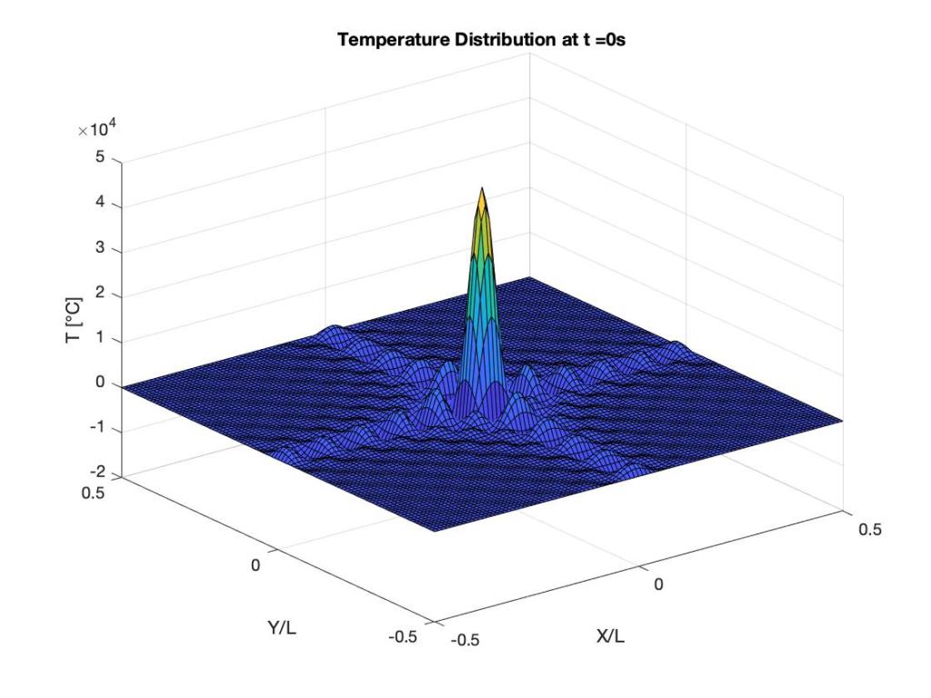
Let us now plot the solution and observe its evolution. From the offset, we see that the whole solution decays with time at a rate of $latex \alpha \lambda_{mn}^2$.
The solution below is for the following conditions:
\[ L = 10m, W = 10m, T_{plasma} = 10000^{\circ}C, \alpha_{steel} = 1.172e^{-5} m^2/s\]
 |
|---|
 |
 |
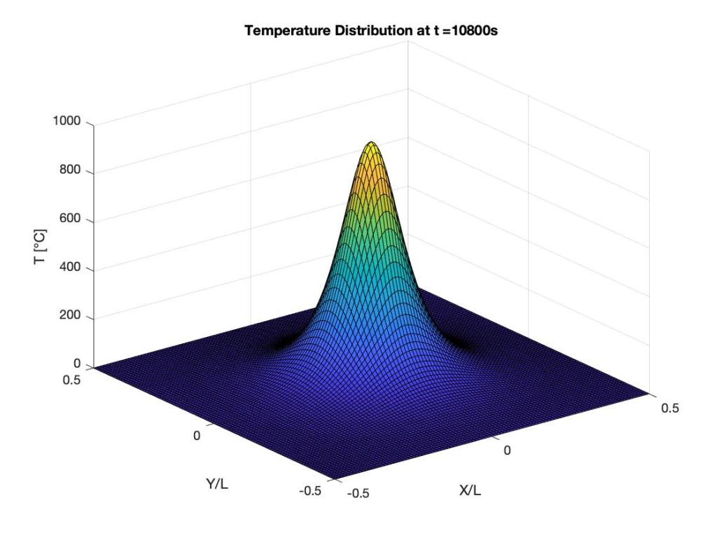 |
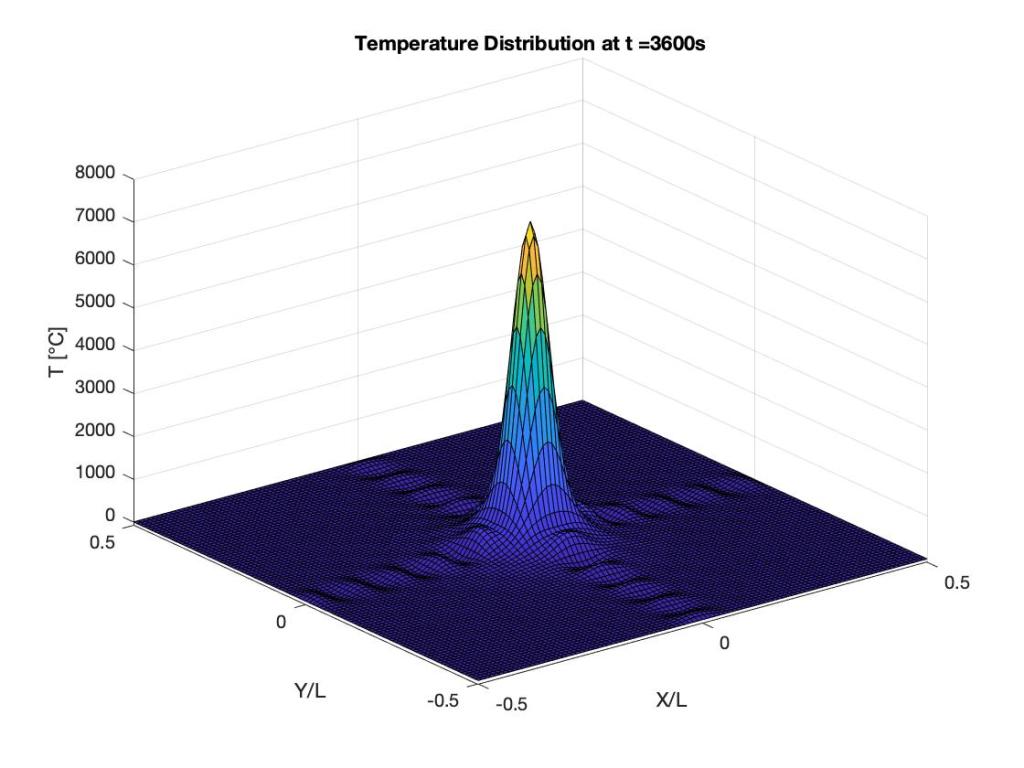
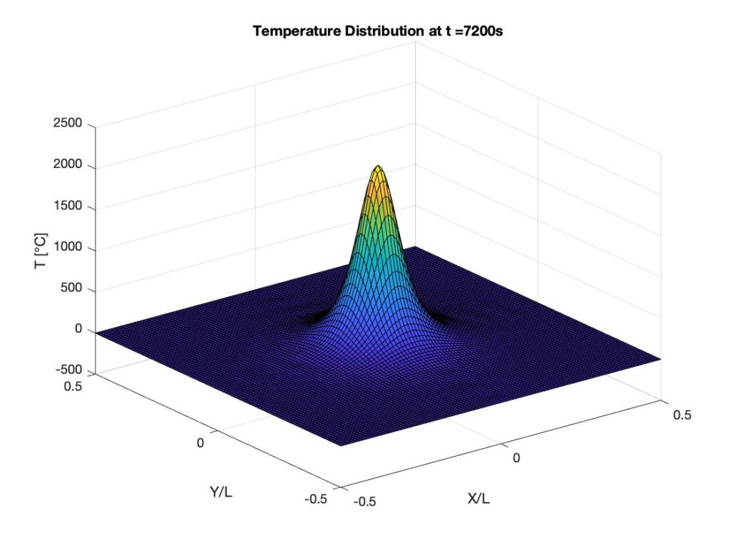
| Temperature Distribution for a Steel plate 10mx10m exposed to an extremely high temperature impulse. |
The solution shows the decaying. You can see this by observing the maximum values on the temperature axis. The initial solution is extremely wavy in nature because of the initial singularity. As the solution progresses, we see a smooth solution which decays with time.
Let’s look at the physical ramifications of this. We can see the temperature gradients set up at the initial instant. The thermal stresses set up will extremely large, which will certainly cause structural failure. Let us look forward in time. 1 hours later, the temperature is still of the order $latex 10^3$. It is pretty obvious that steel by this point would have melted.
Till the time we cannot create a material that can withstand this high temperature, in my opinion, we should not go ahead with fusion. However rare this occurrence might be, we cannot risk another Chernobyl or Fukushima. There are other alternatives that we need to explore in the mean time which could meet our needs.
Author’s Note: This work presents why fusion may not work assuming a catastrophic failure of the magnets keeping the plasma away from the walls of the reactor. As noted in various other research works, a small number of particles breaking away from the plasma will not destroy a reactor as they do not contain enough energy. While temperature (surrogate for energy) of the particle is large, since the particle is very small, it’s energy is actually very small (remember, Boltzmann Constant $latex k_B \sim 10^{-23}$. Thus, even at $latex T = 10^6$, the energy is not enough to affect the first wall). Further, I am willing to back fusion if someone can prove it to me that such an occurrence is extremely rare.