Solving 2-D Diffusion using Strum-Liouville Equations
Sturm-Liouville Equations are a set of second-order linear differential equations that are given by:
\[ \displaystyle \dfrac {d}{dx} [p(x) \dfrac{dy}{dx}] + q(x)y = -\lambda w(x)y \]
where \( y\) is a function of \( x\), and \( p(x), q(x)\) and \( w(x)\) are known, continuously differentiable functions of \( x\) over the region \( (a,b)\).
Sturm-Liouville equations are commonly observed in solving applied mathematical problems, especially in heat transfer and fluid dynamics problems. While they look extremely complicated, there is a hidden beauty in these equations which makes their solutions elegant.
In the above equation, \( \lambda \) represents the eigenvalues of the problem including the boundary conditions. The corresponding solutions are called the eigenfunctions.
Some important knowledge about eigenvalues and eigenfunctions with respect to the Sturm-Liouville problems is given below:
- \( \lambda_1 < \lambda_2 < \lambda_3 < … < \lambda_n\) as \( n\rightarrow \infty \); i.e. the eigenvalues are arranged in an ascending order.
- Eigenvalues are unique, and each correspond to an eigenfunction. For each \( \lambda_n\), \( y_n(x)\) has exact \( (n-1)\) zeros in \( (a,b)\). \( y_n(x)\) is referred to as the \( nth\) zero of the Sturm-Liouville problem.
- All eigenfunctions are normal to each other. Mathematically,
\( \displaystyle \int_a^b y_m(x)y_n(x)w(x)dx = \delta_{mn}\)
The above text has been referenced from Wikipedia. I will subsequently try to build an intuition for a non-expert to spot these equations and solve them with confidence.
One of the most common equations observed in applied mathematics is the Laplace equation. The Laplace equation is given by:
\[ \displaystyle \Delta u = 0 \]
In 1-D, this becomes:
\[ \dfrac{d^2 u}{dx^2} = 0\]
This has a direct solution by integrating twice. The solution is given by:
\[ u = C_1 x + C_2\]
where C1 and C2 are obtained from the boundary conditions given for the problem.
If we look closely, we see that the differential equation is the diffusion equation in 1D. This is the same equation we would solve if we wanted to solve a 1D conduction problem without internal heat generation.
Expanding this to 2D,
\[ \dfrac{{\partial}^2 u}{\partial x^2} + \dfrac{{\partial}^2 u}{\partial y^2} = 0\]
This equation is solved using the concept of separation of variables, which is generally introduced in a calculus class. The concept involves stating that \( \displaystyle u \) is a product of two functions- each function being only dependent on one independent variable. This idea of separating the solution into two functions works because of the inherent nature of the separation. The separation allows us to break down the problem into independent sub-problems that are equal to a constant. Solving these sub-problems while satisfying the boundary values will lead the full solution.
In any case, let
\[ u = X(x).Y(y)\]
Substituting this in the above equation will show us something remarkable:
\[ Y(x)\dfrac{{\partial\ }^2 X(x)}{\partial x^2} + X(x)\dfrac{{\partial\ }^2 Y(y)}{\partial y^2} = 0\]
Dividing by \( u = X(x).Y(y)\), and rearranging,
\[ \dfrac{1}{Y(x)} . \dfrac{{\partial\ }^2 Y(y)}{\partial y^2} = -\dfrac{1}{X(x)} . \dfrac{{\partial\ }^2 X(x)}{\partial x^2} \]
Since the left hand side and right hand side are function of different independent variables, and are equal, they must be equal to a constant. Let that constant by \( \displaystyle \lambda^2\).
In theory, the sign preceding \( \displaystyle \lambda^2\) must be such that it produces a Sturm-Liouville Problem in the direction that has all homogeneous boundary condition. If readers are interested in knowing more about how this works out, I would refer them to some wonderful resources namely: Heat Conduction, by Ozisik, explanation by Professor Sanjiva Lele (ICME, Stanford), and Wikipedia.
Assuming the following boundary conditions:
\[ u(x = 0, y) = 0\]
\[ u(x = L, y) = 0\]
\[ u(x, y = 0) = 0\]
\[ u(x, y = W) = 1\]
From above, we have:
\[ \dfrac{1}{Y(x)} . \dfrac{{\partial\ }^2 Y(y)}{\partial y^2} = -\dfrac{1}{X(x)} . \dfrac{{\partial\ }^2 X(x)}{\partial x^2} = \lambda^2 \]
i.e.
\[ \dfrac{{\partial\ }^2 Y(y)}{\partial y^2} - \lambda^2.Y(y) = 0\]
and
\[ \dfrac{{\partial\ }^2 X(x)}{\partial x^2} + \lambda^2.X(x) = 0\]
The solutions to the above are:
\[ \displaystyle X(x) = C_1\cos(\lambda x) + C_2\sin(\lambda x)\]
\[ Y(y) = C_3\cosh(\lambda y) + C_4\sinh(\lambda y)\]
Thus,
\[ u = (C_1\cos(\lambda x) + C_2\sin(\lambda x))(C_3\cosh(\lambda y) + C_4\sinh(\lambda y))\]
Applying the boundary conditions,
\[ u(x = 0, y) = (C_1)(C_3\cosh(\lambda y) + C_4\sinh(\lambda y)) \Rightarrow C_1 = 0\]
\[ u(x = L, y) = (C_2\sin(\lambda L))(C_3\cosh(\lambda y) + C_4\sinh(\lambda y)) \Rightarrow sin(\lambda L) = 0 \Rightarrow \lambda = \dfrac{n\pi}{L}, n = 0, 1, 2, …\]
\[ u_n(x, y = 0) = (C_2\sin(\lambda_n x))(C_3) \Rightarrow C_3 = 0\]
Thus,
\[ u_n(x, y) = C_2\sin(\lambda_n x)C_4\sinh(\lambda_n y)\]
\[ u_n(x, y) = C_n\sin(\lambda_n x)\sinh(\lambda_n y)\]
So the full solution to the problem is given by,
\[ u(x,y) = \displaystyle\sum\limits_{n = 0}^{\infty} C_n\sin(\lambda_n x)\sinh(\lambda_n y)\]
Using the last boundary condition now,
\[ \displaystyle u(x, y = W) = \displaystyle\sum\limits_{n = 0}^{\infty} C_n\sin(\lambda_n x)\sinh(\lambda_n W)\]
i.e. \[ \displaystyle 1 = \sum\limits_{n = 0}^{\infty} a_n\sin(\lambda_n x)\]
Using concepts of orthogonality, we can multiply both sides by \( \displaystyle *\int_{x = 0}^{x = L} \sin(\lambda_m x)dx\).
Thus,
\[ \displaystyle \int_{x = 0}^{x = L} \sin(\lambda_m x)dx = \displaystyle\int_{x = 0}^{x = L} \displaystyle\sum\limits_{n = 0}^{\infty} a_n\sin(\lambda_n x)\sin(\lambda_m x)dx\]
The right side, due to orthogonality will be non-zero only when \( \displaystyle m = n\). Thus,
\[ \displaystyle \int_{x = 0}^{x = L} \sin(\lambda_n x)dx = a_n\displaystyle\int_{x = 0}^{x = L} \sin^2(\lambda_n x)dx\]
\[ \displaystyle \therefore a_n = \dfrac{\displaystyle\int_{x = 0}^{x = L} \sin(\lambda_n x) dx}{\displaystyle\int_{x = 0}^{x = L} \sin^2(\lambda_n x)dx}\]
\[ \displaystyle \Rightarrow C_n = \dfrac{\displaystyle\int_{x = 0}^{x = L} \sin(\lambda_n x) dx}{\sinh(\lambda_n W) \displaystyle\int_{x = 0}^{x = L} \sin^2(\lambda_n x)dx}\] where \( \displaystyle \lambda_n = \dfrac{n\pi}{L}\).
The full solution thus is given by:
\[ \displaystyle u(x, y) = \sum\limits_{n = 0}^{\infty} \dfrac{\displaystyle\int_{x = 0}^{x = L} \sin(\lambda_n x) dx}{\sinh(\lambda_n W) \displaystyle\displaystyle\int_{x = 0}^{x = L} \sin^2(\lambda_n x)dx} \sin(\lambda_n x)\sinh(\lambda_n y)\] where \( \displaystyle \lambda_n = \dfrac{n\pi}{L} \)
 |
After so much cumbersome math, the question one should ask is what on earth does all this mean physically. Yes, the math is pretty but if it has no physical meaning, it is of no use to us. So let us try to unwrap the physical meaning of our solution.
Let us first look at the solution at boundaries. As we would expect, the solution should agree with the boundary conditions we imposed on the problem. If they don’t, our solution is wrong.
Starting with \( x = 0\), \( u(0,y) = 0\) as \( \sin(\lambda_n * 0) = 0 \) always, thus satisfying the first boundary condition. Further, at \( x = L\), \( u(L,y) = 0\) as \( \sin(\lambda_n * L) = \sin(\dfrac{n\pi}{L}L) = \sin(n\pi) = 0\) always, thus satisfying the second boundary condition.
Now, looking at \( y = 0\), \( u(x,0) = 0\) as \( \sinh(\lambda_n * 0) = 0\) always, thus satisfying the third boundary condition. Now, at \( y = W\), \( u(x,W) = \displaystyle \sum_{n=0}^{\infty} \dfrac{\displaystyle\int_{x=0}^{x=L} \sin(\lambda_n x)dx}{\displaystyle\int_{x=0}^{x=L} \sin^2(\lambda_nx)dx} \sin(\lambda_nx)\). This needs to be further simplified.
Let us first look at \( \displaystyle\int_{x=0}^{x=L}\sin(\lambda_nx)dx\). Replacing \( \lambda_n = \dfrac{n\pi}{L}\), we have \( \displaystyle \int_{x=0}^{x=L}\sin(\dfrac{n\pi x}{L})dx = \dfrac{L}{n\pi} [(-1)^{n+1} + 1]\).
Next, looking at \( \displaystyle \int_{x=0}^{x=L}\sin^2(\lambda_nx)dx\). Replacing \( \lambda_n = \dfrac{n\pi}{L}\), we have \( \displaystyle \int_{x=0}^{x=L}\sin^2(\dfrac{n\pi x}{L})dx = \dfrac{L}{2}\).
Now, looking at the full term, we have:
\[ u(x,W) = \displaystyle \sum_{n=0}^{\infty} \dfrac{\dfrac{L}{n\pi} ((-1)^{n+1} + 1)}{\dfrac{L}{2}} \sin(\lambda_nx)\]
\[ \therefore u(x,W) = \displaystyle \dfrac{2}{\pi}\sum_{n=0}^{\infty}\dfrac {[(-1)^{n+1} + 1]}{n} \sin(\dfrac{n\pi x}{L})\]
This is a Fourier series expansion for \( f(x) = \text{sgn(x)}\). The Fourier series for \( \text{sgn(x)} = \displaystyle \dfrac{2}{\pi}\sum_{n=0}^{\infty}\dfrac {((-1)^{n+1} + 1]}{n} \sin(\dfrac{n\pi x}{L})\). In our domain, \( x \in (0,L)\). Thus, the \( \text{sgn(x)} = 1\). The proof for the Fourier expansion is left to the readers.
\[ \therefore u(x,W) = 1\]
Thus, we have successfully proved the boundary conditions for the problem are satisfied by our solution. Now, let us understand what this means physically inside the domain.
If we were to fix the value of \( y\), the solution will form a sum of sines for each location of \( x\).
\[ u(x,y=constant) = \displaystyle\sum\limits_{n = 0}^{\infty} \dfrac{\sinh(\lambda_n y)\displaystyle\int_{x = 0}^{x = L} \sin(\lambda_n x) dx}{\sinh(\lambda_n W) \displaystyle\displaystyle\int_{x = 0}^{x = L} \sin^2(\lambda_n x)dx} \sin(\lambda_n x)\] where \( \displaystyle \lambda_n = \dfrac{n\pi}{L} \).
Rewriting this,
\[ u(x,y=constant) = \displaystyle \sum\limits_{n=0}^{\infty} b_n \sin(\dfrac{n\pi x}{L})\]
This is just the odd part of a Fourier series. Thus, for each value of \( y\), the solution for \( u\) can be described by the odd part of a Fourier series.
Similarly, if we fix the value of \( x\), we will obtain:
\[ u(x=constant,y) = \displaystyle\sum\limits_{n = 0}^{\infty} \dfrac{\sin(\lambda_n x)\displaystyle\int_{x = 0}^{x = L} \sin(\lambda_n x) dx}{\sinh(\lambda_n W) \displaystyle\displaystyle\int_{x = 0}^{x = L} \sin^2(\lambda_n x)dx} \sinh(\lambda_n y)\] where \( \displaystyle \lambda_n = \dfrac{n\pi}{L} \).
Rewriting this,
\[ u(x=constant,y) = \displaystyle \sum\limits_{n=0}^{\infty} a_n \sinh(\dfrac{n\pi x}{L})\]
This is a sum of hyperbolic sines.
Doing this allows us to see that the solution has spatial frequencies. In a continuous sense, these frequencies do not carry much physical meaning. However in the discrete world, these frequencies govern how fast information is being transferred. This is critical in establishing the numerical stability of a method.
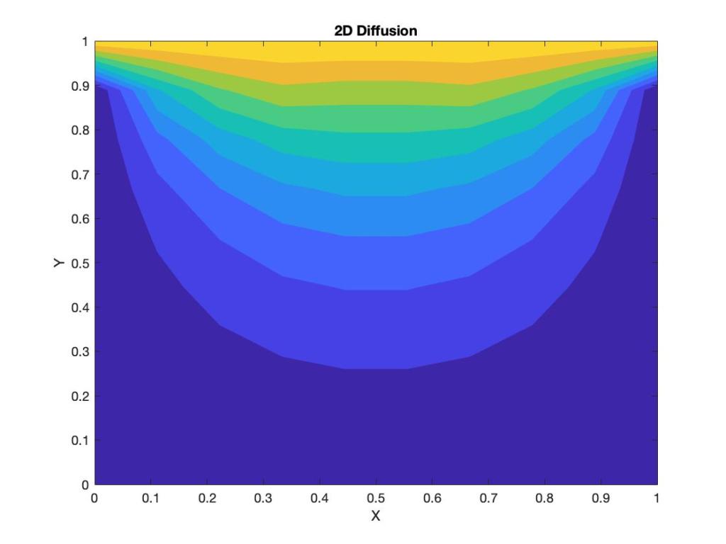
Further, also observe that \( \displaystyle \dfrac{\partial u}{\partial x} \Biggr\vert_{x = \frac{L}{2}}= 0\). Thus, for all values of \( y\), the peak of \( u\) will occur at \( x = \dfrac{L}{2}\) within the domain.
Thus, we now saw how we can solve the Laplace equation using the Sturm-Liouville formulation and what the solution means physically.