Appreciating the Fluid Equations
 |
|---|
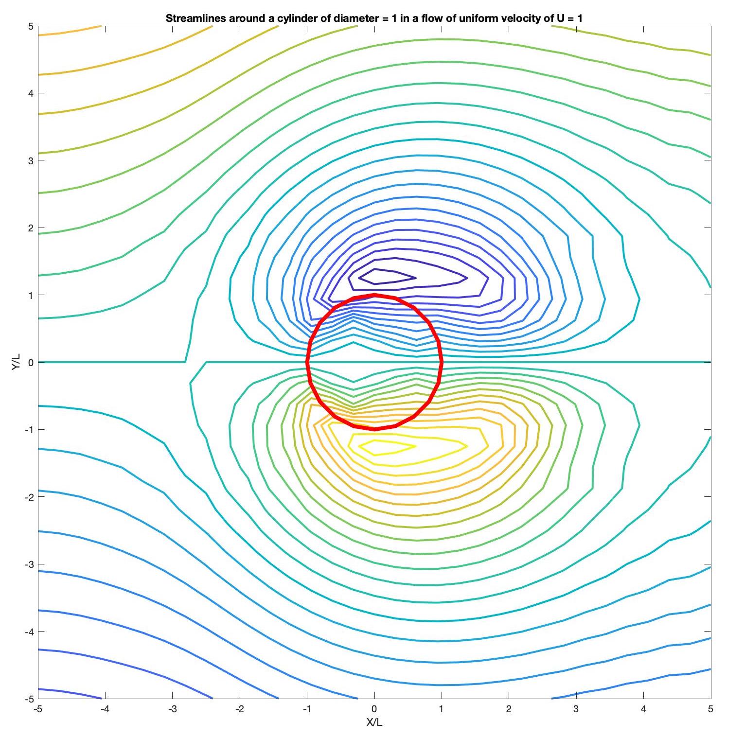
| Streamlines around a cylinder of diameter = 1 in a flow of uniform velocity of U = 1. Note here that the diameter and velocity are non-dimensionalized, and thus do not have any units. |
Computational Fluid Dynamics (CFD) is one of my favorite fields of study. Many times I am asked why, and my answer is fairly simple. CFD merges the two things I am very passionate about: computers and fluids.
To be able to visualize fluid flows has been one of the most important ways I have learnt to love and appreciate the almost arcane equations of fluid dynamics. The Navier-Stokes equations describe all fluid flows (in general cases). In an incompressible flow, these equations take the form of:
\[ \frac{\partial\textbf{u}}{\partial t} + \textbf{u}.{\nabla\textbf{u}} = -\frac{1}{\rho} \nabla p + \nu \Delta\textbf{u} + \textbf{g} \]
The beauty of this equation is it describes motions of the fluid in 3 dimensions and time. All of this information is packed into one compact form that is stated above. Another important equation for fluid motions in continuity:
\[ \nabla \cdot \textbf{u} = 0\]
While the Navier-Stokes describes the motion of the fluid, the continuity equation ensure that the volume of the fluid does not increase of decrease throughout its motion.
These equations seem daunting on first glance, don’t they? There are bunch of things happening in there that you may or may not encountered before. While a standard fluid dynamics text book will do a far better job at explaining the actual physical meaning of each term, I want to point out some of the more mathematical aspects of these equations and then translate them into the physical world.
Let us first decipher the simpler continuity equation. From the wikipedia definition of the continuity equation, “A continuity equation in physics is an equation that describes the transport of some quantity.” In our case, some quantity would refer to the fluid.
The continuity equation in fluid dynamics for incompressible flows states that the velocity of the fluid will be divergence free, i.e. the velocity field is solenoidal. In layman terms, this means that the velocity will only be affected by changes in the flow due to obstructions. If there are no obstruction, the velocity will remain the same.
A very common case when we see this is when we want to increase the velocity of the water coming out of a pipe, we put our thumb across the opening of the pipe. This reduces the area available for the water to flow into. And since water is incompressible, it speeds up and comes out of the pipe at a faster velocity.
Now let us focus on the Navier-Stokes equation. To a mathematician, the Navier-Stokes equation will come off as an elegant second order, non-linear, time dependent partial differential equation in three dimensions. Thats a bunch of terms that I will unbundle step by step. But before that, I want to take some time to mention what each term of the equation actually represents in a mathematical setting.
Partial differential equations (specifically linear partial differential equations) can be classified into three types: hyperbolic, parabolic and elliptic. Hyperbolic equations are related to motions of waves, parabolic equations are related to time-dependent diffusion and elliptic equations are for steady-state diffusion.
In the Navier-Stokes equation, we have the following:
- Elliptic/Parabolic Part
\[ \frac{\partial\textbf{u}}{\partial t} = \nu\Delta\textbf{u} \]
This form the parabolic part of the Navier-Stokes equation. Note how this equation has a very close resemblance to the heat diffusion equation for macroscopic conduction. Under steady state, we can ignore the partial derivative with time and we end up with an elliptic partial differential equation.
Classic heat conduction problems can be solved by separation of variables or using the Green’s function method. Either way, these equations have been solved countless times analytically and agree with the experimental results.
- Non-linear Hyperbolic Part
\[ \frac{\partial \textbf{u}}{\partial t} + \textbf{u}.\nabla\textbf{u} = 0 \]
This form the non-linear hyperbolic part of the Navier-Stokes equation. This equation describes how velocity would be advected away. The hyperbolic part comes from the fact that the above equation is one of the roots to the general form of the hyperbolic partial differential equation. The non-linear nature comes in because of the velocity is dotted with the gradient of itself.
Grouping these ideas together, we have a complex equation with terms that describe abstract ideas for fluid flow. While these are not the most complicated equations one will ever encounter, solving these equations analytically without simplifying assumptions or conditions is next to impossible. Thats the beauty: elegant equations that seem arcane and yet form the foundation of so many things around us.
This is why CFD is one of my favorite fields to study. CFD allows me to solve this equations in an approximate form, and yield some highly accurate results which I can visualize. As a visual learner, CFD has been an extremely useful tool to aid my learning experience.